Understanding L2 Regularization in Artificial Neural Networks (ANN)

In this article, we’ll take a look at L2 Regularization in Artificial Neural Networks (ANN) with code using tensorflow library. Using this regularization technique, we can resolve the issues like overfitting in neural networks.

Table of Contents

Overview

Artificial Neural Networks (ANN) are powerful models used in machine learning for a wide range of tasks, including classification, regression, and pattern recognition. However, ANN can be prone to overfitting, where the model learns to memorize the training data rather than generalize from it. To address this issue, regularization techniques are employed, one of which is L2 regularization. In this article, we’ll explore what L2 regularization is, why it’s important, and how it can be implemented in ANN with a simple code example with sklearn library. We are gonna make use of make_moons toy dataset from sklearn.

What is L2 Regularization ?

L2 regularization, also known as weight decay, is a technique used to prevent overfitting in ANN by adding a penalty term to the loss function. This penalty term is proportional to the square of the L2 norm of the weights in the model. In simpler terms, L2 regularization encourages the weights of the model to be small, effectively simplifying the model and reducing its tendency to overfit the training data.

Overfitting occurs when a model learns to capture noise or irrelevant patterns in the training data, leading to poor generalization performance on unseen data. L2 regularization helps prevent overfitting by discouraging the model from learning overly complex representations of the data. By penalizing large weights, L2 regularization encourages the model to focus on the most important features of the data and reduces its sensitivity to noise.

About Toy Dataset

The make_moons dataset is a synthetic toy dataset generator provided by the scikit-learn library, which is commonly used for practicing and testing machine learning algorithms. This dataset is designed to generate a simple binary classification problem in the shape of two interleaving half circles, hence the name “moons“.

Implementation of L2 Regularization in ANN

Here our only goal is to implement L2 regularization in ANN using TensorFlow. First things first, import all libraries and dependencies.

import numpy as np
import matplotlib.pyplot as plt
from sklearn.datasets import make_moons
import seaborn as sns
from mlxtend.plotting import plot_decision_regions

import tensorflow
from tensorflow.keras.models import Sequential
from tensorflow.keras.layers import Dense
from tensorflow.keras.layers import Dropout
from tensorflow.keras.optimizers import Adam

Separate input and output data columns in X and y numpy array variables. As you can see we added some noise to our data (around 0.25) and took 100 rows.

X, y = make_moons(100, noise=0.25,random_state=2)

Let’s see the datapoints using scatter plot graph.

import matplotlib.pyplot as plt
plt.scatter(X[:,0], X[:,1], c=y)
plt.show()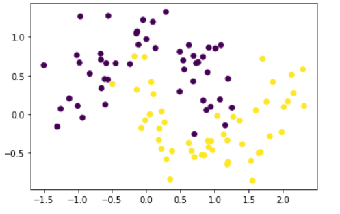

We have to perform classification on this data and we’ll make ANN to do this. We’ll create two neural networks here, one without regularization (model1) and second with regularization parameter (model2). First create model without regularization parameter and name it as model1.

model1 = Sequential()

model1.add(Dense(128,input_dim=2, activation="relu"))
model1.add(Dense(128, activation="relu"))
model1.add(Dense(1,activation='sigmoid'))

Here in above code, we took one input layer with 2 input dimensions, two hidden layers with 128 nodes(neurons) each and ‘relu‘ as activation function. We also have one output layer with only one node and ‘sigmoid‘ as activation function. We usually use sigmoid on output layer in binary classification problems.

Lets show the summary for this model1.

model1.summary()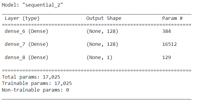

We have total 17025 trainable parameters.

Now lets compile and train our model quickly.

adam = Adam(learning_rate=0.01)
model1.compile(loss='binary_crossentropy', optimizer=adam, metrics=['accuracy'])

history1 = model1.fit(X, y, epochs=2000, validation_split = 0.2,verbose=0)

In above code, we first set the learning rate as 0.01 using Adam optimizer, Then compile our model1 with ‘binary_crossentropy‘ as loss function. We are going with 2000 epochs here intentionally so that there will be overfitting in model. Plus the validation split while training is 0.2.

If we can plot the graph of each region, it would look like this.

plot_decision_regions(X, y.astype('int'), clf=model1, legend=2)
plt.xlim(-2,3)
plt.ylim(-1.5,2)
plt.show()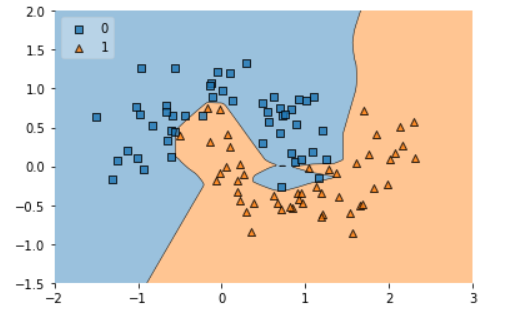

As we can see in above graph, there is clearly lot of overfitting is happening in data (decision boundary). Our model is trying to memories all data points instead of generalize from it. We can also see this overfitting issue using plotting the difference between loss and validation loss like below graph.

plt.plot(history1.history['loss'])
plt.plot(history1.history['val_loss'])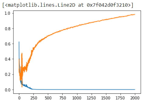

So, to overcome this overfitting issue we need to add regularization term in our neural network. Lets create another model name model2 with regularization parameter in it.

model2 = Sequential()

model2.add(Dense(128,input_dim=2, activation="relu",kernel_regularizer=tensorflow.keras.regularizers.l2(0.03)))
model2.add(Dense(128, activation="relu",kernel_regularizer=tensorflow.keras.regularizers.l2(0.03)))
model2.add(Dense(1,activation='sigmoid'))

Here everything is same as before, we just added the “kernel_regularizer” from tensorflow as 0.03(lambda value). Now lets check the summary for it as well.

model2.summary()

Now compile model2 and train it as we done before for model1.

adam = Adam(learning_rate=0.01)
model2.compile(loss='binary_crossentropy', optimizer=adam, metrics=['accuracy'])

history2 = model2.fit(X, y, epochs=2000, validation_split = 0.2,verbose=0)

If we check the decision regions now, it would look more generalize than before. Take a look on below graph.

plot_decision_regions(X, y.astype('int'), clf=model2, legend=2)
plt.xlim(-2,3)
plt.ylim(-1.5,2)
plt.show()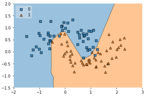

Also the difference between loss and validation loss is minimize.

plt.plot(history2.history['loss'])
plt.plot(history2.history['val_loss'])

So we can conclude that the second model2 will perform better on unseen data as there is very less overfitting issues now.

We can convey the same point using graph PDF(probability density function) like below.

model1_weight_layer1 = model1.get_weights()[0].reshape(256)
model2_weight_layer1 = model2.get_weights()[0].reshape(256)

sns.distplot(model1_weight_layer1)
sns.distplot(model2_weight_layer1)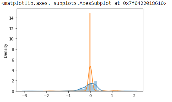

On the above graph, the blue curve is without regularization, and orange curve is with regularization and you can see the regularization curve lies very near to zero value. You can try the same thing with L1 regularization as well.

L2 regularization is a valuable technique in ANN for preventing overfitting and improving generalization performance. By penalizing large weights, L2 regularization encourages simpler models that are less prone to memorizing noise in the training data.