Data modeling is nothing but bringing multiple tables together and drawing relationships between them to create right reports and dashboards.
Overview
Knowing how semantic models are set up is like having a map to create the best model for your reports and dashboards. There are different ways to build a semantic model, but some ways are better than others. The best models are crucial because they make sure your queries run quickly, and your data refreshes don’t take too long. Plus, they use fewer resources like memory and CPU, which means you can have more models without it costing too much. It’s like building a really efficient system to make your work easier!
Data Modeling is like making a plan for your data. It’s about creating a blueprint that shows how data is structured, what it looks like, and how different pieces relate to each other. Imagine you’re building a puzzle, and each piece represents a part of your data. To create this plan, you connect different parts or entities that make sense in a given situation. There are various types of data models, like the Hierarchical Model, Relational Model, Network Model, Dimensional Model, and more.
Concepts to Learn For Data Modeling
- Why Does Data Modeling Matter in Power BI
- Normalization and Denormalization
- Star Schemas
- Fact tables
- Dimension tables
- Fundamental Relationship Concepts
- Cardinality
- Cross Filter Direction
- Active and Inactive Relationships
Why Does Data Modeling Matter in Power BI
- It support efficient data exploration. Users can quickly navigate through data.
- Imagine your data model is like a traffic system. If it’s poorly designed, with lots of confusing connections and repeated information (like having the same road in multiple places), it’s going to slow down the flow of traffic. In the data world, this means your queries (questions you ask your data) might take a long time to get answers, causing delays in showing your reports. So, just like a well-planned road system keeps traffic moving smoothly, a well-designed data model helps your data flow quickly and keeps your reports loading fast.
- It makes future maintainability much easier.
Normalization and Denormalization
To understand some star schema concepts described in this article, it’s important to know two terms: normalization and denormalization.
Normalization, it is the process of dividing larger tables into smaller tables and linking them using relationships.
Denormalization is the opposite of normalization. Instead of splitting tables, you combine them into one table. You might wonder why we need denormalization if normalization exists. One of the major reasons for denormalizing data is to optimize system performance.
Let’s talk about making things simpler for Power BI. Normalization is like organizing your stuff neatly. It reduces the size of your tables, making it quicker to find things. Think of it like having a well-arranged bookshelf – everything in its place, easy to grab. Now, if you have a huge, messy table (imagine a jumbled-up pile of books), finding what you need takes longer.
But, there’s also a concept called denormalization. This comes into play when dealing with more complex data structures, like snowflake dimensions and junk dimensions. It’s like temporarily spreading your books across a big table for a specific task, then putting them back neatly. So, in Power BI, we choose between keeping things organized (normalized) for everyday ease or spreading things out for specific tasks (denormalized). It’s about finding the right balance.
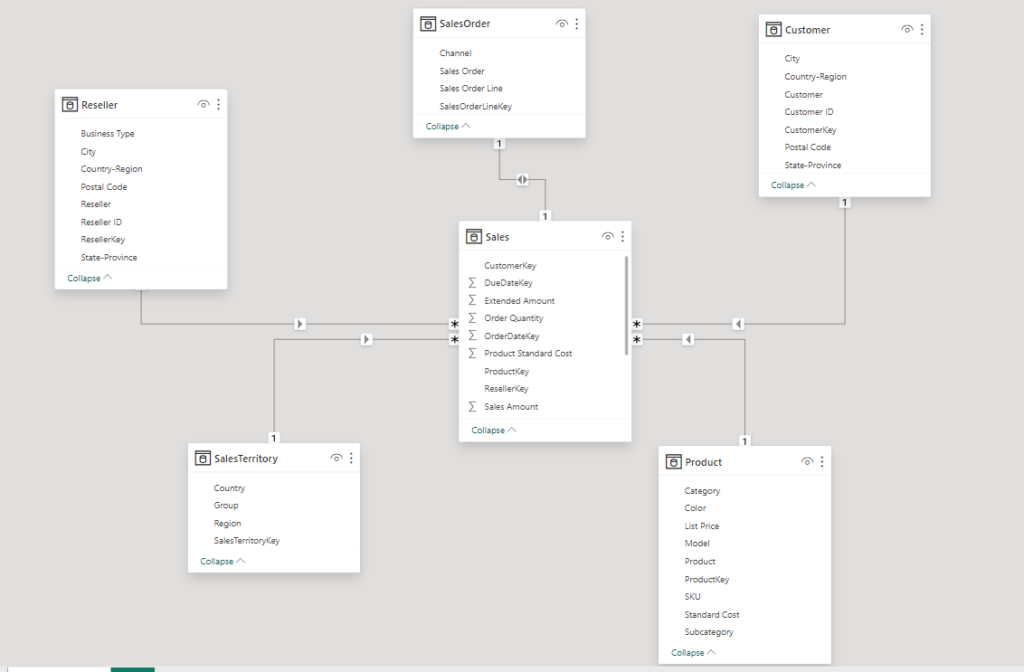
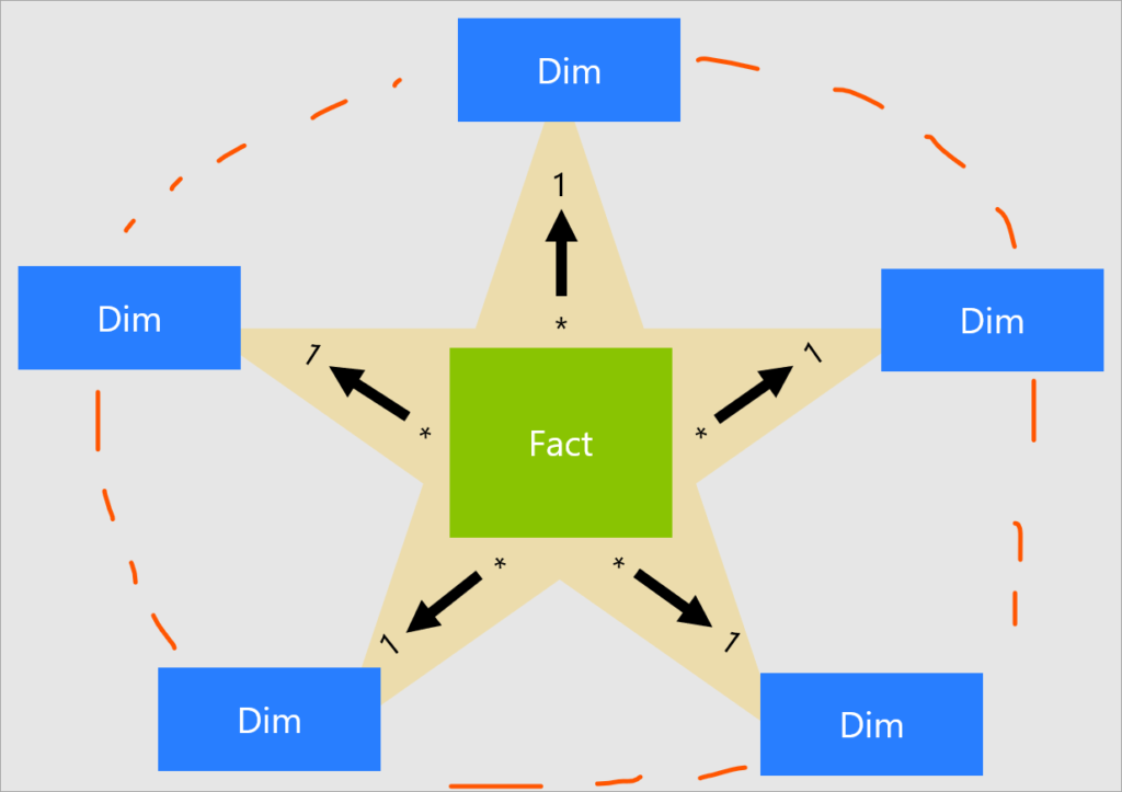
Star Schemas
Alright, let’s break it down! Imagine you’re organizing your room. In a star schema, you neatly separate your things into two groups: the important stuff (let’s call them dimensions, like types of furniture) and the action stuff (those are the facts, like what you do in your room). It’s like having well-labeled drawers and a big to-do list. Star schemas de-normalize the data, which means adding redundant columns to some dimension tables.
Now, there’s another way – a single flat table schema. It’s like dumping everything into one giant box. But for Power BI, this isn’t the best move. It’s like trying to find your socks, your books, and your snacks all in one messy pile. So, stick with the star schema – it keeps things tidy and makes it easier to find what you need.
Fact Tables
Also known as Data or Master table. Think of a fact table as your treasure chest for numbers! This special table in Power BI is like your vault where you keep all the important data that can be counted and analyzed. Each row in the table is like a golden ticket that tells a story about a specific event or transaction.
Picture a sales fact table – it’s like a magical list that shows when a sale happened, what product was sold, how many were sold, and how much money rolled in. Every column in this table is like a key detail that helps you uncover valuable insights about your data. So, the fact table is your go-to spot for all the important numerical info in Power BI. It has foreign key and support summarization.
Dimension Tables
Also known as Lookup or Mapping table. Think of a dimension table as your trusty guide that adds all the juicy details to the numbers in your fact table! If the fact table is like a treasure chest full of numbers, the dimension table is like the map that tells you exactly where each treasure is located.
For example, if you have a sales fact table that shows how much was sold, a product dimension table would give you more info about each product, like its name, category, description, and even the supplier’s name. Dimension tables are like the sidekicks that make your data more interesting and easier to understand.
Even though dimension tables are smaller in size, they’re a crucial part of the data model. They’re linked to the fact table, forming a powerful duo that lets you dig into the data, filter it, group it, and uncover valuable insights with ease. It has primary key and supports filtering and grouping.
Fundamental Relationship Concepts
Primary and Foreign Keys
Keys are like the secret code that connects tables in a data dance! A primary key in one table matches with a foreign key in another, making them a perfect pair. It’s the way tables share info and keep everything in sync.
Primary Key
Think of a primary key as a VIP pass for each row in a table. It’s a special column or group of columns that holds a unique code for every row. No two rows can have the same code. It’s like giving each row a personal ID card that makes them stand out in the crowd. The primary key’s distinct count equals the number of rows in the table.
Foreign Key
Also known as alternative key, an alternative key is a column in a table whose values correspond to the values of a primary key in another table.
Cardinality
Our fact and dimension tables connect via primary and alternative keys, but we must define their relationship further. Each relationship in a model is defined by a cardinality type. It refers to the number of unique values in one table related to the number of unique values in another.
There are three types of cardinality relationships in Power BI data modeling.
One-to-One (1:1)
This occurs when one record in the first table is related to one and only one record in the second table. This type of relationship is relatively rare in Power BI data modeling.
One-to-Many (1:N)
This occurs when one record in the first table can be related to many records in the second table, and it is the most common type of relationship in Power BI data modeling. This cardinality type is used to link a fact table with one or more dimension tables, where the dimension table is typically on the “one” side of the relationship, and the fact table generally is on the “many” side. The one-to-many and many-to-one cardinality options are essentially the same.
Many-to-Many (N:N)
This occurs when many records in the first table can be related to many records in the second table. This relationship type is not directly supported in Power BI data modeling and is infrequently used.
Knowing how tables are linked (the cardinality) is crucial in Power BI. It affects how data behaves in your reports how it groups, filters, and shows up visually. Understanding this connection is key to making your reports work just right!
Cross Filter Direction in Data Modeling
Relationships in your model have a filter direction: either single (one-way) or both (two-way). This influences how filters flow between tables. Understanding this helps you control how your data responds when you’re building reports in Power BI.
Single
In a single-directional cross filter, filtering in one table affects the other, but not vice versa. It’s like a one-way street for filters in your Power BI data model.
Bi-Directional
In a bi-directional cross filter, filters can flow in both directions, impacting data in both tables. However, it’s less common due to potential performance issues and filter ambiguity.
The possible cross-filter options are dependent on the cardinality type. Relationships with a 1:1 cardinality can only have a bi-directional cross-filter direction, whereas One:Many and Many:Many relationships can have either single or bi-directional cross-filter directions.
Active and Inactive Relationships
In Power BI, tables are joined and filtered based on active relationships by default. However, when dealing with multiple relationships between tables, it’s crucial to designate one as active while others remain inactive to prevent conflicts and ensure accurate results.
Points to Remember
- There can be only one active relationship between two tables.
- We mostly prefer ‘Star Schema’ and ‘One-to-many’ cardinality.
- Primary key is in Dimensional table, and Foreign key is in Fact table.
- Primary key has unique values, foreign key has duplicate values.
- Always calendar date table categorized as ‘Dimensions’.