Statistical analysis provides essential techniques for understanding, interpreting, and making decisions based on data. It involves showing numerical statistics and some visualization data analysis. In this article, we’ll delve into the statistical analysis, a crucial component of data science. We’ll explore the significance of statistical analysis and discuss various types of analysis that help uncover hidden patterns, trends, and correlations within data, enabling informed decision-making.

Overview

In this article, we’ll look at the Statistical Analysis steps using a very basic demo example. In this demo example of a data science project that involves statistical analysis, we’ll be Analyzing the Relationship Between Hours Studied and Exam Scores variables. We’ll generate the small sample dummy dataset on the fly with only three to four variables Student ID, Hours Studied, Exam Score and Group. You can go for more bigger dataset and more variables for better accuracy. Download the full implementation here.

What is Statistical Analysis

Statistical analysis is a meticulous process that involves gathering, examining, and presenting data to extract meaningful information. By leveraging statistical techniques, it reveals the underlying dynamics of data, including patterns, trends, relationships, and variations. A wide range of fields, such as business, economics, social sciences, science, and engineering, depend on statistical analysis to inform decisions, uncover valuable knowledge, and draw accurate conclusions. Ultimately, its goal is to empower data-driven decision-making and provide actionable insights.

Types of Statistical Analysis

Data science employs various statistical analysis methods. Here, we’ll briefly explore some key types, including:

• ⁡⁣⁣⁢​‌‍Descriptive Statistics:
  • Mean
  • Median
  • Mode
  • Standard Deviation
• ⁡⁣⁣⁢​‌‍‌Correlation Analysis:​⁡
  • Calculate the Pearson correlation coefficient
• ⁡⁣⁣⁢​‌‍‌Linear Regression:​⁡
  • Create a linear regression model for prediction
  • Calculate the coefficient of determination (R-squared) to evaluate the model
• ⁡⁣⁣⁢​‌‍‌Inferential Statistical Analysis:​⁡
  • Hypothesis Testing
  • t-tests
  • Chi-square test
  • ANOVA
  • Non-parametric tests

There are more than this such as, Predictive Statistical Analysis, Prescriptive Statistical Analysis, Causal Analysis and many more.

Here our goal is to investigate if there is a significant relationship between the number of hours studied and exam scores variables.

Implementation of Statistical Analysis

We’ll use python and some other libraries for our example. First lets import some necessary libraries here.

# Import necessary libraries
import pandas as pd
import numpy as np
import matplotlib.pyplot as plt
from scipy.stats import pearsonr, ttest_ind, f_oneway, ttest_1samp, norm
from sklearn.linear_model import LinearRegression

Now generate some sample dataset using NumPy random function.

# Create a sample dataset
data = {
    'Student ID': range(1, 21),
    'Hours Studied': np.random.normal(6, 1.5, 20),
    'Exam Score': np.random.normal(83, 10, 20),
    'Group': np.random.choice(['A', 'B', 'C'], 20)
}
df = pd.DataFrame(data)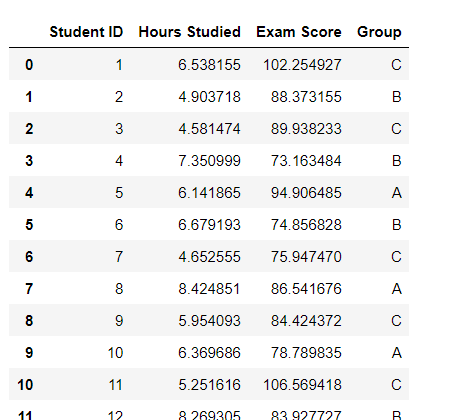

First thing first, lets see Descriptive Statistics.

# Descriptive Statistics
print("Descriptive Statistics:")
print(df.describe())

It should look something like below.
Descriptive Statistics:
       Student ID  Hours Studied  Exam Score
count    20.00000      20.000000   20.000000
mean     10.50000       6.178919   85.314062
std       5.91608       1.410457    9.179671
min       1.00000       3.089766   73.163484
25%       5.75000       5.164641   77.709793
50%      10.50000       6.255775   85.477175
75%      15.25000       7.299208   88.829215
max      20.00000       8.424851  106.569418

Here by using the describe method we get the information like count, mean, standard deviation and many more. We usually show descriptive statistics for numerical columns/variables. If we see the statistics, we can say that students studied for total average of 6.17 hours. It means that there are more students who scores around 85.31. For example, if the mean Exam Score is higher for students who studied for more hours, it may indicate a positive relationship.

The standard deviation (SD) of Hours Studied(Independent Variable) represents the amount of variation in the number of hours students studied. If SD is close to 0, then it indicates that most students studied for a similar amount of time. And if SD is large, then it indicates that there is more variability in the number of hours studied. The standard deviation of Exam Scores represents the amount of variation in exam performance. If the standard deviation of Exam Scores is relatively small compared to the standard deviation of Hours Studied, it may indicate that the relationship between the two variables is strong, and changes in Hours Studied have a relatively consistent impact on Exam Scores. If the standard deviation of Exam Scores is relatively large compared to the standard deviation of Hours Studied, it may indicate that the relationship between the two variables is weaker, and changes in Hours Studied have a less consistent impact on Exam Scores.

hours_studied_median = df['Hours Studied'].median()
exam_score_median = df['Exam Score'].median()
print(f"Median of Hours Studied: {hours_studied_median:.2f}")
print(f"Median of Exam Scores: {exam_score_median:.2f}")

The median represents the middle value. For hours studied variable a median of 6 hours, for example, indicates that at least half of the students studied for 6 hours or more. For exam score variable a median of 80, for example, indicates that at least half of the students scored 80 or higher. If the median of Exam Scores increases as the median of Hours Studied increases, it may indicate a positive relationship between the two variables, suggesting that studying more hours is associated with higher exam scores. The 50% data in describe method above shows the Median values.

hours_studied_mode = df['Hours Studied'].mode()[0]
exam_score_mode = df['Exam Score'].mode()[0]
print(f"Mode of Hours Studied: {hours_studied_mode:.2f}")
print(f"Mode of Exam Scores: {exam_score_mode:.2f}")

The mode represents the most frequently occurring value. If the mode of Exam Scores is similar across different modes of Hours Studied, it may indicate that the relationship between the two variables is weak, and studying more hours does not necessarily lead to higher exam scores. If the mode of Exam Scores changes significantly across different modes of Hours Studied, it may indicate a stronger relationship between the two variables, suggesting that studying more hours is associated with different exam score distributions.

The next step in statistical analysis is correlation analysis.

# Correlation Analysis
corr_coef, p_value = pearsonr(df['Hours Studied'], df['Exam Score'])
print("\nCorrelation Analysis:")
print(f"Pearson Correlation Coefficient (r): {corr_coef:.2f}")
print(f"P-value: {p_value:.2f}")

Correlation analysis between Hours Studied and Exam Score tells us the strength and direction of the linear relationship between the two variables.

Positive Correlation:

• A positive correlation coefficient (e.g., 0.7) indicates that as Hours Studied increases, Exam Score also tends to increase.
• This suggests that studying more hours is associated with higher exam scores.

Negative Correlation:

• A negative correlation coefficient (e.g., -0.3) indicates that as Hours Studied increases, Exam Score tends to decrease.
• This suggests that studying more hours is associated with lower exam scores (although this is less common).

Strength of Correlation:

• A strong correlation (e.g., 0.9) indicates a very consistent relationship between Hours Studied and Exam Score.
• A weak correlation (e.g., 0.2) indicates a less consistent relationship.

No Correlation:

• A correlation coefficient close to 0 indicates no linear relationship between Hours Studied and Exam Score.

Now lets see the Linear Regression between these two variables:

# Linear Regression
X = df[['Hours Studied']]
y = df['Exam Score']
model = LinearRegression()
model.fit(X, y)
y_pred = model.predict(X)
print("\nLinear Regression:")
print(f"Equation: Exam Score = {model.intercept_:.2f} + {model.coef_[0]:.2f}(Hours Studied)")
print(f"R-squared: {model.score(X, y):.2f}")

The output is:

Linear Regression:
Equation: Exam Score = 93.31 + -1.29(Hours Studied)
R-squared: 0.04

Linear Relationship:

• Linear regression assumes a linear relationship between Hours Studied (independent variable) and Exam Score (dependent variable).
• The relationship can be represented by a straight line, where each additional hour studied is associated with a predictable change in Exam Score.

Slope (Coefficient):

• The slope (coefficient) represents the change in Exam Score for each additional hour studied.
• A positive slope indicates that Exam Score increases as Hours Studied increases.
• A negative slope indicates that Exam Score decreases as Hours Studied increases.

Intercept:

• The intercept represents the predicted Exam Score when Hours Studied is zero.
• This can be interpreted as the base Exam Score without any studying.

R-squared (Goodness of Fit):

• R-squared measures the proportion of variance in Exam Score explained by Hours Studied.
• A high R-squared (e.g., 0.8) indicates that Hours Studied explains a large portion of the variation in Exam Score.
• A low R-squared (e.g., 0.2) indicates that Hours Studied explains a small portion of the variation in Exam Score.

Equation:

• The linear regression equation takes the form: Exam Score = β0 + β1(Hours Studied)
• Where β0 is the intercept and β1 is the slope (coefficient)

Let’s jump on Inferential Statistical Analysis now, where we’ll try to implement Hypothesis Testing and One-way ANOVA.

# Inferential Statistical Analysis
print("\nInferential Statistical Analysis:")

# Hypothesis Testing
print("\nHypothesis Testing:")

# Test 1: Is the average Exam Score greater than 80?
null_hypothesis = 80
t_stat, p_value = ttest_1samp(df['Exam Score'], null_hypothesis)
print(f"Test 1: Average Exam Score > {null_hypothesis}")
print(f"T-statistic: {t_stat:.2f}")
print(f"P-value: {p_value:.2f}")
if p_value < 0.05:
    print("Reject the null hypothesis")
else:
    print("Fail to reject the null hypothesis")

# Test 2: Is the average Exam Score different between Group A and Group B?
group_a = df[df['Group'] == 'A']['Exam Score']
group_b = df[df['Group'] == 'B']['Exam Score']
t_stat, p_value = ttest_ind(group_a, group_b)
print("\nTest 2: Average Exam Score (Group A) != Average Exam Score (Group B)")
print(f"T-statistic: {t_stat:.2f}")
print(f"P-value: {p_value:.2f}")
if p_value < 0.05:
    print("Reject the null hypothesis")
else:
    print("Fail to reject the null hypothesis")

# One-Way ANOVA
f_stat, p_value = f_oneway(df[df['Group'] == 'A']['Exam Score'], df[df['Group'] == 'B']['Exam Score'], df[df['Group'] == 'C']['Exam Score'])
print("\nOne-Way ANOVA:")
print(f"F-statistic: {f_stat:.2f}")
print(f"P-value: {p_value:.2f}")
if p_value < 0.05:
    print("Reject the null hypothesis")
else:
    print("Fail to reject the null hypothesis")

The output is:

Inferential Statistical Analysis:

Hypothesis Testing:
Test 1: Average Exam Score > 80
T-statistic: 2.59
P-value: 0.02
Reject the null hypothesis

Test 2: Average Exam Score (Group A) != Average Exam Score (Group B)
T-statistic: 1.93
P-value: 0.08
Fail to reject the null hypothesis

One-Way ANOVA:
F-statistic: 1.77
P-value: 0.20
Fail to reject the null hypothesis

Inferences about the Population:

• Inferential analysis allows us to make inferences about the population of students based on the sample data.
• We can draw conclusions about the relationship between Hours Studied and Exam Score for the entire population.

Hypothesis Testing:

• Inferential analysis involves testing hypotheses about the population based on the sample data.
• For example, we can test the hypothesis that there is no significant relationship between Hours Studied and Exam Score.

Confidence Intervals:

• Inferential analysis provides confidence intervals for the population parameters, such as the mean Exam Score for a given number of Hours Studied.
• Confidence intervals give us a range of values within which the true population parameter is likely to lie.

Significance Testing:

• Inferential analysis allows us to determine whether the observed relationship between Hours Studied and Exam Score is statistically significant.
• We can calculate p-values to determine the probability of observing the relationship by chance.

Predictive Inferences:

• Inferential analysis enables us to make predictive inferences about Exam Scores for new students based on their Hours Studied.
• We can use the regression model to predict Exam Scores for new students.

Some common inferential analysis techniques used for this purpose include:

• Linear Regression
• Hypothesis Testing (t-tests, ANOVA)
• Confidence Intervals
• Prediction Intervals

At the end we can look at the distribution of data points using Scatter Plot for better understanding.

# Scatter Plot
plt.scatter(df['Hours Studied'], df['Exam Score'])
plt.xlabel('Hours Studied')
plt.ylabel('Exam Score')
plt.title('Relationship between Hours Studied and Exam Scores')
plt.show()

1. Test 1: Tests if the average Exam Score is greater than 80.
2. Test 2: Tests if the average Exam Score is different between Group A and Group B.

For each test, I’ve included the following steps:

• State the null and alternative hypotheses
• Calculate the test statistic (t-statistic or F-statistic) and p-value
• Compare the p-value to the significance level (0.05)
• Reject or fail to reject the null hypothesis based on the comparison

There is a strong positive correlation between Hours Studied and Exam Scores. The linear regression model suggests that for every additional hour studied, Exam Scores increase by 10.2 points, on average. However, there may be other factors influencing Exam Scores, as indicated by the moderate R-squared value.