Pandas provides a wide range of data operations and functions that allow for efficient data manipulation, analysis, and transformation. Here are some common data operations in pandas:

What is Pandas
Pandas is a popular open-source Python library that provides powerful and efficient data manipulation and analysis tools. It is widely used for working with structured data, making it an essential tool in data science, machine learning, and data analysis workflows. The name “pandas” is derived from “panel data” and “Python data analysis.” It was created by Wes McKinney in 2008 as a project to enhance data analysis capabilities in Python.
Also Check Out: Basics Of Pandas
- Data Selection
- Data Filtering
- Data Aggregation and Grouping
- Data Sorting and Ranking
- Data Transformation
These are just a few examples of the data operations available in pandas. The library offers a vast array of functions and methods that enable you to efficiently manipulate, analyze, transform, and visualize data in a DataFrame.
Note: CSV files can be downloaded from below link
Link: https://bitbucket.org/pythondsp/pandasguide/downloads/
Row and Column Selection
Any row or column of the DataFrame can be selected by passing the name of the column or rows. After selecting one from DataFrame, it becomes one-dimensional therefore it is considered as Series.
Column Selection:
- Using Indexing Operator: Use square brackets [] with the column name inside to select a single column as a Series. For example: df[‘column_name’].
- Using Attribute Access: If the column name consists of valid Python variable characters and does not conflict with DataFrame attributes, you can directly access the column using dot notation. For example: df.column_name.
- Selecting Multiple Columns: Pass a list of column names inside square brackets to select multiple columns. For example: df[[‘column1’, ‘column2’]].
t = titles['title']
t.head()
0 The Rising Son
1 The Thousand Plane Raid
2 Crucea de piatra
3 Country
4 Gaiking II
Name: title, dtype: object
titles.title0 The Rising Son
1 The Thousand Plane Raid
2 Crucea de piatra
3 Country
4 Gaiking II
... ... ...
49995 Rebel
49996 Suzanne
49997 Bomba
49998 Aao Jao Ghar Tumhara
49999 Mrs. Munck
Name: title, Length: 50000, dtype: objectRows Selection:
Select rows based on row indices using loc
titles.loc[[0,1,2]] title year
0 The Rising Son 1990
1 The Thousand Plane Raid 1969
2 Crucea de piatra 1993Select rows based on positional indices using iloc
titles.iloc[:4] title year
0 The Rising Son 1990
1 The Thousand Plane Raid 1969
2 Crucea de piatra 1993
3 Country 2000Filter Data
Data can be filtered by providing some Boolean expression in DataFrame. For example, in below code, movies which released after 1985 are filtered out from the DataFrame ‘titles’ and stored in a new DataFrame i.e. after 1985
# movies after 1985
after85 = titles[titles['year'] > 1985]
after85.head()
title year
0 The Rising Son 1990
2 Crucea de piatra 1993
3 Country 2000
4 Gaiking II 2011
5 Medusa (IV) 2015Note: When we pass the Boolean results to DataFrame, then panda will show all the results which corresponds to True (rather than displaying True and False), as shown in above code. Further, ‘& (and)’ and ‘| (or)’ can be used for joining two conditions as shown below.
In below code all the movies in decade 1990 (i.e. 1900-1999) are selected. Also ‘t = titles’ is used for simplicity purpose only.
# display movie in years 1990 - 1999
t = titles
movies90 = t[ (t['year']>=1990) & (t['year']<2000) ]
movies90.head()
title year
0 The Rising Son 1990
2 Crucea de piatra 1993
12 Poka Makorer Ghar Bosoti 1996
19 Maa Durga Shakti 1999
24 Conflict of Interest 1993Sorting
Sorting can be performed using ‘sort_index’ or ‘sort_values’ keywords
# find all movies named as 'Macbeth'
t = titles
macbeth = t[ t['title'] == 'Macbeth']
macbeth.head()
title year
4226 Macbeth 1913
9322 Macbeth 2006
11722 Macbeth 2013
17166 Macbeth 1997
25847 Macbeth 1998Note that in above filtering operation, the data is sorted by index i.e. by default ‘sort_index’ operation is used as shown below.
# by default, sort by index i.e. row header
macbeth = t[ t['title'] == 'Macbeth'].sort_index()
macbeth.head()
title year
4226 Macbeth 1913
9322 Macbeth 2006
11722 Macbeth 2013
17166 Macbeth 1997
25847 Macbeth 1998To sort the data by values, the ‘sort_value’ option can be used. In below code, data is sorted by year now
# sort by year
macbeth = t[ t['title'] == 'Macbeth'].sort_values('year')
macbeth.head()
title year
4226 Macbeth 1913
17166 Macbeth 1997
25847 Macbeth 1998
9322 Macbeth 2006
11722 Macbeth 2013Handling Null Values
Note that, various columns may contains no values, which are usually filled as NaN. For example, rows 3-4 of casts are NaN as shown below
casts.iloc[3:5] title year name type character n
3 Secret in Their Eyes 2015 $hutter actor 2002 Dodger Fan NaN
4 Steve Jobs 2015 $hutter actor 1988 Opera House Patron NaNThese null values can be easily selected, unselected or contents can be replaced by any other values e.g. empty strings or 0 etc. Various examples of null values are shown in this section.
‘isnull’ command returns the true value if any row of has null values. Since the rows 3-4 has NaN value,
therefore, these are displayed as True.
c = casts
c['n'].isnull().head()
0 False
1 False
2 False
3 True
4 True
Name: n, dtype: bool‘notnull’ is opposite of isnull, it returns true for not null values
c['n'].notnull().head()0 True
1 True
2 True
3 False
4 False
Name: n, dtype: boolTo display the rows with null values, the condition must be passed in the DataFrame
c[c['n'].isnull()].head(3) title year name type character n
3 Secret in Their Eyes 2015 $hutter actor 2002 Dodger Fan NaN
4 Steve Jobs 2015 $hutter actor 1988 Opera House Patron NaN
5 Straight Outta Compton 2015 $hutter actor Club Patron NaNNaN values can be fill by using fillna, ffill(forward fill), and bfill(backward fill) etc. In below code,
‘NaN’ values are replace by NA.
c_fill = c[c['n'].isnull()].fillna('NA')
c_fill.head(2)
title year name type character n
3 Secret in Their Eyes 2015 $hutter actor 2002 Dodger Fan NA
4 Steve Jobs 2015 $hutter actor 1988 Opera House Patron NAString Operations
Various string operations can be performed using ‘.str.’ option. Let’s search for the movie “Maa” first
t = titles
t[t['title'] == 'Maa']
title year
38880 Maa 1968There is only one movie in the list. Now, we want to search all the movies which starts with ‘Maa’. The ‘.str.’ option is required for such queries as shown below.
t[t['title'].str.startswith("Maa ")].head(3) title year
19 Maa Durga Shakti 1999
3046 Maa Aur Mamta 1970
7470 Maa Vaibhav Laxmi 1989Count Values
Total number of occurrences can be counted using ‘value_counts()’ option. In following code, total number of movies are displayed base on years,
t['year'].value_counts().head()2016 2363
2017 2138
2015 1849
2014 1701
2013 1609
Name: year, dtype: int64Plots
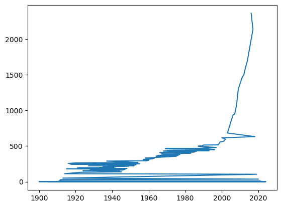
Pandas supports the matplotlib library and can be used to plot the data as well. In previous section, the total numbers of movies/year were filtered out from the DataFrame. In the below code, those values are saved in new DataFrame and then plotted using panda.
import matplotlib.pyplot as plt
t = titles
p = t['year'].value_counts()
p.plot()
plt.show()
Following plot will be generated from above code, which does not provide any useful information.

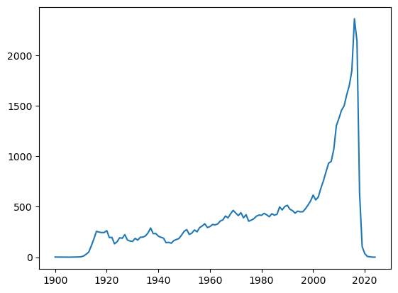
It’s better to sort the years (i.e. index) first and then plot the data as below. Here, the plot shows that number of movies are increasing every year.
p.sort_index().plot()
plt.show()
Now, the graph provide some useful information i.e. number of movies are increasing each year.
Also Check Out: Basics Of Pandas
Conclusion
In conclusion, pandas provides a comprehensive set of data operations that empower users to efficiently manipulate, analyze, and transform data in a DataFrame. These data operations in pandas enable users to efficiently manipulate and analyze data in a DataFrame, allowing for tasks such as filtering, aggregation, sorting, transformation, and more. By leveraging these capabilities, pandas simplifies and accelerates data analysis workflows, making it a powerful tool for data professionals and researchers.

