This tutorial focuses on developing a system designed to identify images of cats and dogs using CNN. It involves analyzing various images containing cats and dogs to predict which animal is present in each image. To train the system, the Dogs vs Cats dataset, accessible through Kaggle, is utilized. This dataset consists of numerous images that enable the model to learn and recognize the unique characteristics and traits associated with cats and dogs. We can access the dataset here.
Learning Objectives
- Get started with Convolutional Neural Networks (CNNs) for image classification.
- Master image data preprocessing and augmentation with Keras and TensorFlow.
- Understand CNN architecture: convolutional, activation, pooling, and fully connected layers.
- Hands-on experience building a CNN model to classify cat and dog images using the Dogs vs Cats dataset.
Understanding Convolutional Neural Networks (CNNs)
Convolutional Neural Networks (CNNs) are a class of deep learning models specifically designed for processing and analyzing visual data, such as images. Unlike traditional neural networks, CNNs leverage convolutional layers to automatically learn hierarchical features from the input data.
The Architecture of a CNN for Cat and Dog Classification
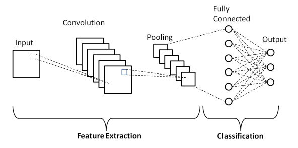
A typical CNN architecture for cat and dog classification consists of several convolutional layers followed by max-pooling layers to ‘downsample‘ the feature maps and reduce spatial dimensions. These layers are often interleaved with activation functions, such as ‘ReLU‘, to introduce non-linearity and increase the model’s representational power. After several convolutional and max-pooling layers, the feature maps are flattened and fed into one or more fully connected (dense) layers, which perform high-level feature extraction and classification. The output layer usually consists of a single neuron with a sigmoid activation function, producing a probability score indicating the likelihood of the input image being either a cat or a dog.
Training the CNN Model
Import below libraries:
- NumPy- For working with arrays, linear algebra.
- Pandas – For reading/writing data
- Matplotlib – to display images
- TensorFlow Keras models – Need a model for prediction
- TensorFlow Keras layers – Every NN needs layers and CNN needs well a couple of layers.
For this task, first we’ll directly get data from Kaggle using python code like below. To do this we need to go to the Kaggle profile first and download the API token from account section. This is the kaggle.json file.
#create the folder name kaggle
!mkdir -p ~/.kaggle
!cp kaggle.json ~/.kaggle/
After creating the folder name kaggle, we need to put this kaggle.json file in it and then run the below command to download everything to your system from kaggle. We can find this below API command on kaggle only.
!kaggle datasets download -d salader/dogs-vs-catsNow that we have our downloaded dataset with us, but it is in zip format. We need to unzip this dataset using below code.
import zipfile
zip_ref = zipfile.ZipFile('/content/dogs-vs-cats.zip', 'r')
zip_ref.extractall('/content')
zip_ref.close()
Once we unzip the data, we get train and test data folders.
Import libraries like below.
import tensorflow as tf
from tensorflow import keras
from keras import Sequential
from keras.layers import Dense,Conv2D,MaxPooling2D,Flatten,BatchNormalization,Dropout
Create a generator here to process large amount of data. The generator breaks down the large data into equal size batches and feed it to the RAM to process one by one. In this way the processing of large data becomes easier. We are creating training and validation sub-datasets. The name of this generator from keras is ‘image_dataset_from_directory‘.
# generators
train_ds = keras.utils.image_dataset_from_directory(
    directory = '/content/train',
    labels='inferred',
    label_mode = 'int',
    batch_size=32,
    image_size=(256,256)
)

validation_ds = keras.utils.image_dataset_from_directory(
    directory = '/content/test',
    labels='inferred',
    label_mode = 'int',
    batch_size=32,
    image_size=(256,256)
)
In above code we have converted the image size into 256 x 256. Our train dataset have 20000 files and test dataset have 5000 files. Now we need to normalize the data because our images are stored in Numpy array and it is in values of 0 to 255. We need to normalize it into 0 to 1 for easy processing.
# Normalize
def process(image,label):
    image = tf.cast(image/255. ,tf.float32)
    return image,label

train_ds = train_ds.map(process)
validation_ds = validation_ds.map(process)
Create an model with three convolution layers. We are implementing max pooling after each convolution layers. We have implemented the three fully connected layers as well.
# create CNN model

model = Sequential()

model.add(Conv2D(32,kernel_size=(3,3),padding='valid',activation='relu',input_shape=(256,256,3)))
model.add(BatchNormalization())
model.add(MaxPooling2D(pool_size=(2,2),strides=2,padding='valid'))

model.add(Conv2D(64,kernel_size=(3,3),padding='valid',activation='relu'))
model.add(BatchNormalization())
model.add(MaxPooling2D(pool_size=(2,2),strides=2,padding='valid'))

model.add(Conv2D(128,kernel_size=(3,3),padding='valid',activation='relu'))
model.add(BatchNormalization())
model.add(MaxPooling2D(pool_size=(2,2),strides=2,padding='valid'))

model.add(Flatten())

model.add(Dense(128,activation='relu'))
model.add(Dropout(0.1))
model.add(Dense(64,activation='relu'))
model.add(Dropout(0.1))
model.add(Dense(1,activation='sigmoid'))
Look at the summary.
model.summary()- Total params: 14,848,193
- Trainable params: 14,847,745
- Non-trainable params: 448
Now compile the model using ‘Adam‘ as a optimizer and ‘binary cross entropy‘ as loss function.
model.compile(optimizer='adam',loss='binary_crossentropy',metrics=['accuracy'])Train the model using fit() method.
history = model.fit(train_ds,epochs=10,validation_data=validation_ds)Check accuracy and loss curve for issues like overfitting. If there is overfitting, then we can make the changes.
plt.plot(history.history['accuracy'],color='red',label='train')
plt.plot(history.history['val_accuracy'],color='blue',label='validation')
plt.legend()
plt.show()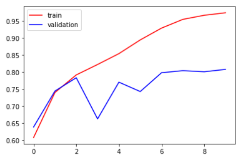
plt.plot(history.history['loss'],color='red',label='train')
plt.plot(history.history['val_loss'],color='blue',label='validation')
plt.legend()
plt.show()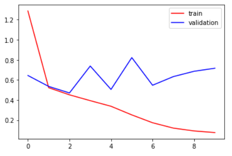
There is little overfitting issue is happening. Below are some ways to reduce overfitting issues. You can try it on your own and make changes to the below items.
- Add more data
- Data Augmentation
- L1/L2 Regularization
- Dropout
- Batch Norm
- Reduce complexity
Now that our model is ready to do the prediction, we’ll make use of new unseen image of cat and dog to do this.
import cv2

test_img = cv2.imread('/content/cat.jpg')
plt.imshow(test_img)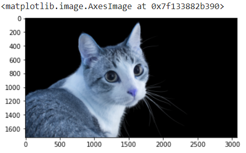
Here first we need to resize the image into 256 x 256 size before doing the prediction.
test_img = cv2.resize(test_img,(256,256))
test_input = test_img.reshape((1,256,256,3))

model.predict(test_input)
array([[0.]], dtype=float32)
In our model output 1 shows the dog and output 0 shows the cat image. You can access full code here.
Convolutional Neural Networks (CNNs) offer a powerful approach to the classification of images, including the classification of cats and dogs. By automatically learning hierarchical features from raw pixel data, CNNs can effectively discriminate between different categories of images with high accuracy.