
Scikit-learn (sklearn) is a popular machine learning library in Python that provides a wide range of tools for building and evaluating machine learning models. Sklearn includes several metrics for evaluating the performance of classification, regression, and clustering models.
We can divide sklearn metrics into three mainly parts:
- Classification Metrics
- Regression Metrics
- Clustering Metrics
Classification Metrics
- Accuracy score:
Accuracy score is a metric used to evaluate the performance of a classification model. It measures the proportion of correctly classified instances out of the total number of instances. In other words, accuracy tells us how often the model’s predictions match the actual labels.
Here’s how accuracy score is calculated:
Accuracy = Total Number of Predictions / Number of Correct Predictions
Let’s illustrate accuracy score with an example:
Suppose we have a binary classification problem where we want to predict whether emails are spam or not spam. We have a dataset with 100 emails, and we build a classification model that predicts whether each email is spam or not spam.
| Email ID | Actual Label | Predicted Label |
|---|---|---|
| 1 | Not Spam | Not Spam |
| 2 | Spam | Spam |
| 3 | Not Spam | Not Spam |
| … | … | … |
| 99 | Spam | Not Spam |
| 100 | Not Spam | Not Spam |
In this example, let’s assume that our model correctly predicted 90 out of 100 emails. That is, it correctly classified 85 emails as not spam and 5 emails as spam.
Number of Correct Predictions = 85 + 5 = 90
Total Number of Predictions =100
Now, we can calculate the accuracy score:
Accuracy = 90/100 = 0.9
So, the accuracy score of our model is 0.9 or 90%. This means that our model correctly classified 90% of the emails in the dataset.
Code:
from sklearn.datasets import load_iris
from sklearn.model_selection import train_test_split
from sklearn.neighbors import KNeighborsClassifier
from sklearn.metrics import accuracy_score

# Load the Iris dataset
iris = load_iris()
X, y = iris.data, iris.target

# Split the data into training and testing sets
X_train, X_test, y_train, y_test = train_test_split(X, y, test_size=0.2, random_state=42)

# Initialize the KNN classifier
knn = KNeighborsClassifier()

# Fit the classifier to the training data
knn.fit(X_train, y_train)

# Make predictions on the test data
y_pred = knn.predict(X_test)

# Calculate accuracy score
accuracy = accuracy_score(y_test, y_pred)

print("Accuracy Score:", accuracy)
- Precision Score
Precision score is a metric used to evaluate the performance of a classification model, particularly in binary classification tasks. It measures the proportion of true positive predictions among all positive predictions made by the model. In other words, precision tells us how many of the instances predicted as positive by the model are actually positive.
Here’s how precision score is calculated:

Let’s illustrate precision score with an example:
Suppose we have a binary classification problem where we want to predict whether patients have a particular disease based on some medical tests. We have a dataset with 100 patients, and we build a classification model that predicts whether each patient has the disease or not.
| Patient ID | Actual Label | Predicted Label |
|---|---|---|
| 1 | Positive | Positive |
| 2 | Negative | Negative |
| 3 | Positive | Negative |
| …. | …. | …. |
| 99 | Negative | Positive |
| 100 | Positive | Positive |
In this example, let’s assume that our model correctly predicted 80 out of 100 patients who have the disease (true positives) and incorrectly predicted 20 patients as having the disease when they do not (false positives).
Now, we can calculate the precision score:
Precision = 80 / (80+20) = 80 / 100 = 0.8
So, the precision score of our model is 0.8 or 80%. This means that out of all the instances predicted as positive by the model, 80% of them are actually positive. Precision score is particularly useful in scenarios where false positives are costly or undesirable, such as medical diagnoses or fraud detection.
Code:
from sklearn.datasets import make_classification
from sklearn.model_selection import train_test_split
from sklearn.linear_model import LogisticRegression
from sklearn.metrics import precision_score

# Generate sample data
X, y = make_classification(n_samples=1000, n_features=20, n_classes=2, random_state=42)

# Split data into training and testing sets
X_train, X_test, y_train, y_test = train_test_split(X, y, test_size=0.2, random_state=42)

# Train a logistic regression model
model = LogisticRegression()
model.fit(X_train, y_train)

# Make predictions on test data
y_pred = model.predict(X_test)

# Calculate precision score
precision = precision_score(y_test, y_pred)

print("Precision Score:", precision)
- Recall Score
Recall score, also known as sensitivity or true positive rate, is a metric used to evaluate the performance of a classification model, particularly in binary classification tasks. It measures the proportion of true positive predictions among all actual positive instances. In other words, recall tells us how many of the positive instances in the dataset were correctly identified by the model.
Here’s how recall score is calculated:
Recall = True Positives / (True Positives + False Negatives)
Let’s illustrate recall score with an example:
Suppose we have a binary classification problem where we want to predict whether patients have a particular disease based on some medical tests. We have a dataset with 100 patients.
Let’s assume that out of the 100 patients who actually have the disease, our model correctly predicted 70 of them as having the disease (true positives) and incorrectly predicted 30 patients as not having the disease when they do (false negatives).
Recall = 70 / (70 + 30) = 70 / 100 = 0.7
So, the recall score of our model is 0.7 or 70%. This means that out of all the patients who actually have the disease, our model correctly identified 70% of them. Recall should be interpreted in conjunction with other metrics like precision to get a comprehensive understanding of the model’s performance.
Code:
from sklearn.metrics import recall_score

# True labels
true_labels = [0, 1, 1, 0, 1, 1, 0, 0, 1, 0]

# Predicted labels
predicted_labels = [0, 1, 1, 0, 1, 0, 1, 0, 1, 0]

# Calculate recall score
recall = recall_score(true_labels, predicted_labels)

print("Recall Score:", recall)
- F1 Score
The F1 score is a metric used to evaluate the performance of a classification model, particularly in binary classification tasks. It is the harmonic mean of precision and recall, providing a balanced measure of the model’s performance. The F1 score considers both false positives and false negatives and is useful when the class distribution is imbalanced.
Here’s how the F1 score is calculated:
F1 Score = 2 × ( (Precision * Recall) / (Precision + Recall) )
The F1 score ranges from 0 to 1, where a higher value indicates better performance. A perfect F1 score of 1 means that the model has achieved perfect precision and recall.
Code:
from sklearn.metrics import f1_score

# True labels
true_labels = [0, 1, 1, 0, 1, 1, 0, 0, 1, 0]

# Predicted labels
predicted_labels = [0, 1, 1, 0, 1, 0, 1, 0, 1, 0]

# Calculate F1 score
f1 = f1_score(true_labels, predicted_labels)

print("F1 Score:", f1)
- Confusion Matrix
A confusion matrix is a table that describes the performance of a classification model by comparing actual values with predicted values. It provides a detailed breakdown of the model’s predictions, showing the number of true positives, true negatives, false positives, and false negatives.
A confusion matrix is particularly useful for evaluating the performance of binary classification models but can also be extended to multi-class classification problems.
Here’s how a confusion matrix is structured:
| – | Predicted Positive | Predicted Negative |
|---|---|---|
| Actual Positive | True Positive (TP) | False Negative (FN) |
| Actual Negative | False Positive (FP) | True Negative (TN) |
- True Positive (TP): Positively correctly predicted.
- True Negative (TN): Negatively correctly predicted.
- False Positive (FP): Positively incorrectly predicted.
- False Negative (FN): Negatively incorrectly predicted.
The confusion matrix provides a comprehensive view of the model’s performance, allowing us to analyze its strengths and weaknesses. It can be used to calculate various performance metrics such as accuracy, precision, recall, and F1 score, providing insights into the model’s predictive power and potential areas for improvement.
Code:
from sklearn.metrics import confusion_matrix

# True labels
true_labels = [0, 1, 1, 0, 1, 1, 0, 0, 1, 0]

# Predicted labels
predicted_labels = [0, 1, 1, 0, 1, 0, 1, 0, 1, 0]

# Compute confusion matrix
cm = confusion_matrix(true_labels, predicted_labels)

print("Confusion Matrix:")
print(cm)
- ROC Curve and AUC
Receiver Operating Characteristic (ROC) curve and Area Under the Curve (AUC) are evaluation metrics used to assess the performance of binary classification models. They provide a graphical representation of the trade-off between the true positive rate (sensitivity) and the false positive rate (1 – specificity) at various classification thresholds.
ROC Curve:
- The ROC curve is created by plotting the true positive rate (sensitivity) against the false positive rate (1 – specificity) for different threshold values.
- To construct the ROC curve, we need to calculate the true positive rate (TPR) and false positive rate (FPR) at various threshold values.
- TPR (sensitivity) = TP / (TP + FN)
- FPR (1 – specificity) = FP / (FP + TN)
- By varying the classification threshold (e.g., from 0 to 1), we can calculate TPR and FPR for each threshold value and plot them on the ROC curve.
AUC (Area Under the Curve):
- The AUC represents the area under the ROC curve and provides a single scalar value to measure the overall performance of the classification model.
- AUC ranges from 0 to 1, where a higher value indicates better performance.
- An AUC of 0.5 suggests random guessing (no discrimination), while an AUC of 1 indicates perfect discrimination.
- AUC can be interpreted as the probability that the model will rank a randomly chosen positive instance higher than a randomly chosen negative instance.
- AUC can be calculated using numerical integration or trapezoidal approximation under the ROC curve.
- Log Loss
Log Loss, also known as logarithmic loss or cross-entropy loss, is a widely used evaluation metric for binary and multiclass classification problems. It measures the performance of a classification model by quantifying the accuracy of its probability predictions.
Here’s how Log Loss is calculated:

Where:
- N is the total number of instances in the dataset.
- yi is the actual label (0 or 1 for binary classification, or a vector of probabilities for multiclass classification) for the ith instance.
- yi^ is the predicted probability of the positive class for the ith instance.
Log Loss penalizes incorrect classifications more severely when the model’s confidence is higher. It is logarithmically scaled, so smaller values indicate better performance.
Regression Metrics
- Mean Absolute Error (MAE)
Mean Absolute Error (MAE) is a metric used to evaluate the performance of a regression model. It measures the average absolute difference between the predicted values and the actual values. MAE gives equal weight to all errors, regardless of their direction (positive or negative).
Here’s how Mean Absolute Error (MAE) is calculated:

Where:
- n is the number of samples in the dataset.
- yi is the actual value of the target variable for the ith sample.
- yi^ is the predicted value of the target variable for the ith sample.
- ∣⋅∣ denotes the absolute value.
Code:
from sklearn.datasets import make_regression
from sklearn.model_selection import train_test_split
from sklearn.linear_model import LinearRegression
from sklearn.metrics import mean_absolute_error

# Generate sample data
X, y = make_regression(n_samples=100, n_features=1, noise=10, random_state=42)

# Split data into training and testing sets
X_train, X_test, y_train, y_test = train_test_split(X, y, test_size=0.2, random_state=42)

# Fit a linear regression model
model = LinearRegression()
model.fit(X_train, y_train)

# Make predictions on test data
y_pred = model.predict(X_test)

# Calculate mean absolute error
mae = mean_absolute_error(y_test, y_pred)

print("Mean Absolute Error (MAE):", mae)
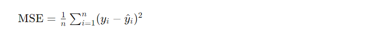
- Mean Squared Error (MSE)
Mean Squared Error (MSE) is a metric used to evaluate the performance of a regression model. It measures the average squared difference between the predicted values and the actual values. MSE penalizes larger errors more heavily than smaller errors, making it sensitive to outliers.
Here’s how Mean Squared Error (MSE) is calculated:
Code:
from sklearn.datasets import make_regression
from sklearn.model_selection import train_test_split
from sklearn.linear_model import LinearRegression
from sklearn.metrics import mean_squared_error

# Generate sample data
X, y = make_regression(n_samples=100, n_features=1, noise=10, random_state=42)

# Split data into training and testing sets
X_train, X_test, y_train, y_test = train_test_split(X, y, test_size=0.2, random_state=42)

# Fit a linear regression model
model = LinearRegression()
model.fit(X_train, y_train)

# Make predictions on test data
y_pred = model.predict(X_test)

# Calculate mean squared error
mse = mean_squared_error(y_test, y_pred)

print("Mean Squared Error (MSE):", mse)
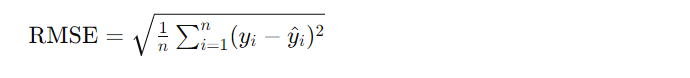
- Root Mean Squared Error (RMSE)
Root Mean Squared Error (RMSE) is a metric used to evaluate the performance of a regression model. It measures the square root of the average squared difference between the predicted values and the actual values. RMSE is a popular metric because it is in the same unit as the target variable, making it interpretable and easy to understand.
Here’s how Root Mean Squared Error (RMSE) is calculated:
Code:
from sklearn.datasets import make_regression
from sklearn.model_selection import train_test_split
from sklearn.linear_model import LinearRegression
from sklearn.metrics import mean_squared_error

# Generate sample data
X, y = make_regression(n_samples=100, n_features=1, noise=10, random_state=42)

# Split data into training and testing sets
X_train, X_test, y_train, y_test = train_test_split(X, y, test_size=0.2, random_state=42)

# Fit a linear regression model
model = LinearRegression()
model.fit(X_train, y_train)

# Make predictions on test data
y_pred = model.predict(X_test)

# Calculate mean squared error
mse = mean_squared_error(y_test, y_pred)

# Calculate RMSE
rmse = mse ** 0.5

print("Root Mean Squared Error (RMSE):", rmse)
- R-squared (R2)
R-squared (R2) is a statistical measure used to assess the goodness-of-fit of a regression model. It indicates the proportion of the variance in the dependent variable that is explained by the independent variables. R-squared values range from 0 to 1, where:
- R2 = 0 indicates that the regression model does not explain any of the variability of the response data around its mean.
- R2 = 1 indicates that the regression model perfectly explains all the variability of the response data around its mean.
Here’s how R-squared (R2) is calculated:
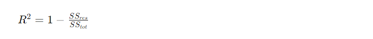
Where:
- SSres is the sum of squares of residuals (the difference between the observed values and the predicted values).
- SStot is the total sum of squares (the difference between the observed values and the mean of the observed values).


Code:
from sklearn.datasets import make_regression
from sklearn.linear_model import LinearRegression
from sklearn.metrics import r2_score

# Generate sample data
X, y = make_regression(n_samples=100, n_features=1, noise=0.1, random_state=42)

# Fit a linear regression model
model = LinearRegression()
model.fit(X, y)

# Make predictions
y_pred = model.predict(X)

# Calculate R2 score
r2 = r2_score(y, y_pred)
print("R-squared (R2) score:", r2)
Clustering Metrics
- Silhouette Score
The Silhouette Score is a metric used to evaluate the clustering performance of a dataset. It quantifies the goodness of clustering by measuring the average distance between clusters and the separation between clusters relative to the within-cluster distance. The Silhouette Score ranges from -1 to 1, where:
- A score close to +1 indicates that the data point is well-clustered and far away from neighboring clusters.
- A score close to 0 indicates that the data point is close to the decision boundary between two neighboring clusters.
- A score close to -1 indicates that the data point may have been assigned to the wrong cluster.
Here’s how the Silhouette Score is calculated for a single data point:
silhouette_coef = (b – a) / max(a, b)
- a is the average distance from the data point to other data points within the same cluster (intra-cluster distance).
- b is the average distance from the data point to the data points in the nearest neighboring cluster (inter-cluster distance).
Compute the silhouette score for the entire dataset:

Code:
from sklearn.datasets import make_blobs
from sklearn.cluster import KMeans
from sklearn.metrics import silhouette_score

# Generate sample data
X, _ = make_blobs(n_samples=1000, centers=3, random_state=42)

# Apply KMeans clustering
kmeans = KMeans(n_clusters=3, random_state=42)
labels = kmeans.fit_predict(X)

# Calculate Silhouette Score
silhouette_avg = silhouette_score(X, labels)
print("Silhouette Score:", silhouette_avg)
- Calinski-Harabasz Index
The Calinski-Harabasz Index (also known as the Variance Ratio Criterion) is a metric used to evaluate the clustering quality of a dataset. It measures both the within-cluster dispersion and the between-cluster dispersion. Higher values of the Calinski-Harabasz Index indicate better-defined clusters.
Code:
from sklearn.datasets import make_blobs
from sklearn.cluster import KMeans
from sklearn.metrics import calinski_harabasz_score

# Generate sample data
X, _ = make_blobs(n_samples=1000, centers=3, random_state=42)

# Apply KMeans clustering
kmeans = KMeans(n_clusters=3, random_state=42)
labels = kmeans.fit_predict(X)

# Calculate Calinski-Harabasz Index
ch_score = calinski_harabasz_score(X, labels)
print("Calinski-Harabasz Index:", ch_score)