In pandas, the groupby() function is used to create groups of data based on one or more columns in a DataFrame. It is a powerful operation that enables various data aggregation and analysis tasks.
Data can be grouped by columns-headers. Further, custom formats can be defined to group the various elements of the DataFrame.
Also Check Out: Basics Of Pandas
Here’s an overview of the groupby() function in pandas:
grouped = df.groupby(by, axis=0, level=None, as_index=True, sort=True, group_keys=True, squeeze=False, observed=False, dropna=True)Parameters
- by: Specifies the column(s) or label(s) by which the DataFrame should be grouped. It can be a single column name or a list of column names.
- axis: Specifies the axis to perform the grouping on. By default, it is set to 0, indicating grouping by rows. Use axis=1 for grouping by columns.
- level: If the DataFrame has a multi-level index, you can specify the level(s) to group by.
- as_index: Specifies whether to use the grouped column(s) as the index of the resulting DataFrame. By default, it is set to True.
- sort: Specifies whether to sort the resulting groups by the group keys. By default, it is set to True.
- group_keys: Specifies whether to include the group keys in the resulting DataFrame index. By default, it is set to True.
- squeeze: Specifies whether to return a DataFrame or a Series when there is only one group. By default, it is set to False.
- observed: Specifies whether to include only observed values in the resulting groups for categorical data. By default, it is set to False.
- dropna: Specifies whether to exclude groups with missing values from the grouping. By default, it is set to True.
Note: CSV files can be downloaded from below link
Link: https://bitbucket.org/pythondsp/pandasguide/downloads/
GroupBy with Column-Names
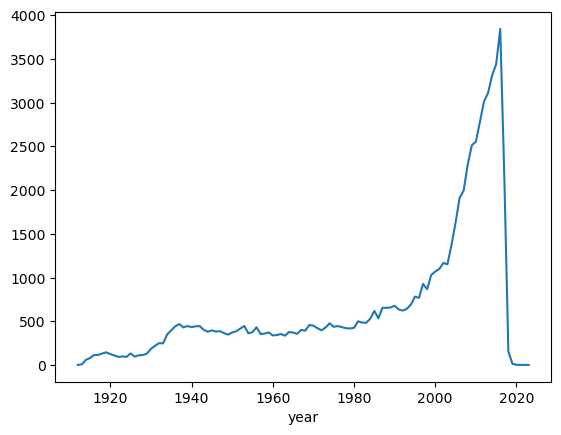
Here Count Values, the value of movies/year were counted using ‘count_values()’ method. Same can be
achieve by ‘groupby’ method as well. The ‘groupby’ command return an object, and we need to an additional functionality to it to get some results. For example, in below code, data is grouped by ‘year’ and then size() command is used. The size() option counts the total number for rows for each year; therefore the result of below code is same as ‘count_values()’ command.
cg = c.groupby(['year']).size()
cg.plot()
plt.show()
Further, groupby option can take multiple parameters for grouping. For example, we want to group the
movies of the actor ‘Aaron Abrams’ based on year.
c = casts
cf = c[c['name'] == 'Aaron Abrams']
cf.groupby(['year']).size().head()
year
2003 2
2004 2
2005 2
2006 1
2007 2
dtype: int64Above list shows that year-2003 is found in two rows with name-entry as ‘Aaron Abrams’. In the other word, he did 2 movies in 2003.
Next, we want to see the list of movies as well, then we can pass two parameters in the list as shown below:
cf.groupby(['year', 'title']).size().head()year title
2003 The In-Laws 1
The Visual Bible: The Gospel of John 1
2004 Resident Evil: Apocalypse 1
Siblings 1
2005 Cinderella Man 1
dtype: int64In above code, the groupby operation is performed on the ‘year’ first and then on ‘title’. In the other word, first all the movies are grouped by year. After that, the result of this groupby is again grouped based on titles. Note that, first group command arranged the year in order i.e. 2003, 2004 and 2005 etc. then next group command arranged the title in alphabetical order.
Next, we want to do grouping based on maximum ratings in a year; i.e. we want to group the items by year and see the maximum rating in those years:
c.groupby(['year']).n.max().head()year
1912 6.0
1913 14.0
1914 39.0
1915 14.0
1916 35.0
Name: n, dtype: float64Above results show that the maximum rating in year 1912 is 6 for Aaron Abrams.
Similarly, we can check for the minimum rating:
c.groupby(['year']).n.min().head()year
1912 6.0
1913 1.0
1914 1.0
1915 1.0
1916 1.0
Name: n, dtype: float64Lastly, we want to check the mean rating each year:
c.groupby(['year']).n.mean().head()year
1912 6.000000
1913 4.142857
1914 7.085106
1915 4.236111
1916 5.037736
Name: n, dtype: float64GroupBy with Custom Field
Suppose we want to group the data based on decades, then we need to create a custom groupby field.
# decade conversion : 1985//10 = 198, 198*10 = 1980
decade = c['year']//10*10
c_dec = c.groupby(decade).n.size()
c_dec.head()
year
1910 669
1920 1121
1930 3448
1940 3997
1950 3892
Name: n, dtype: int64Above results shows the total number of movies in each decade.
What is Unstack in Pandas
Before understanding the unstack, let’s consider one case from cast.csv file. In following code, the data is grouped by decade and type i.e. actor and actress.
Note: CSV files can be downloaded from below link
Link: https://bitbucket.org/pythondsp/pandasguide/downloads/
c = casts
c.groupby( [c['year']//10*10, 'type'] ).size().head(8)
year type
1910 actor 384
actress 285
1920 actor 710
actress 411
1930 actor 2628
actress 820
1940 actor 3014
actress 983
dtype: int64Now we want to compare and plot the total number of actors and actresses in each decade. One solution to this problem is to grab even and odd rows separately and plot the data, which is quite complicated operation if types has more varieties e.g. new-actor, new-actress and teen-actors etc. A simple solution to such problem is the ‘unstack’, which allows to create a new DataFrame based on the grouped Dataframe, as shown below.
Since we want a plot based on actors and actress, therefore first we need to group the data based on ‘type’ as below:
c = casts
c_decade = c.groupby( ['type', c['year']//10*10] ).size()
c_decade
type year
actor 1910 384
1920 710
1930 2628
1940 3014
1950 2877
1960 2775
1970 3044
1980 3565
1990 5108
2000 10368
2010 15523
2020 4
actress 1910 285
1920 411
1930 820
1940 983
1950 1015
1960 968
1970 1299
1980 1989
1990 2544
2000 5831
2010 8853
2020 3
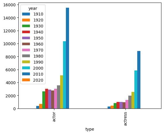
dtype: int64Now we can create a new DataFrame using ‘unstack’ command. The ‘unstack’ command creates a new
DataFrame based on index.
c_decade.unstack()year 1910 1920 1930 1940 1950 1960 1970 1980 1990 ...
type
actor 384 710 2628 3014 2877 2775 3044 3565 5108 ...
actress 285 411 820 983 1015 968 1299 1989 2544 ...c_decade.unstack().plot()
plt.show()
c_decade.unstack().plot(kind='bar')
plt.show()

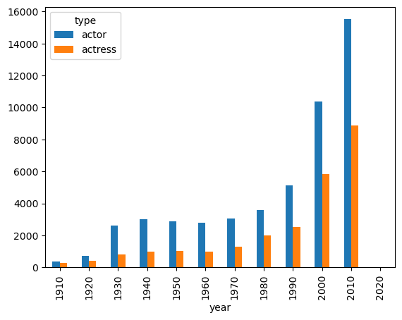
To plot the data side by side, use unstack(0) option as shown below (by default unstack(-1) is used)
c_decade.unstack(0)type actor actress
year
1910 384 285
1920 710 411
1930 2628 820
1940 3014 983
1950 2877 1015
1960 2775 968
1970 3044 1299
1980 3565 1989
1990 5108 2544
2000 10368 5831
2010 15523 8853
2020 4 3c_decade.unstack(0).plot(kind='bar')
plt.show()
Conclusion
In conclusion, the groupby() function in pandas is a powerful tool for grouping data in a DataFrame based on one or more columns. The groupby() function in pandas is a fundamental tool for data analysis and exploration. It enables you to gain insights into the underlying patterns and relationships within your data by grouping and aggregating it based on specific criteria.

